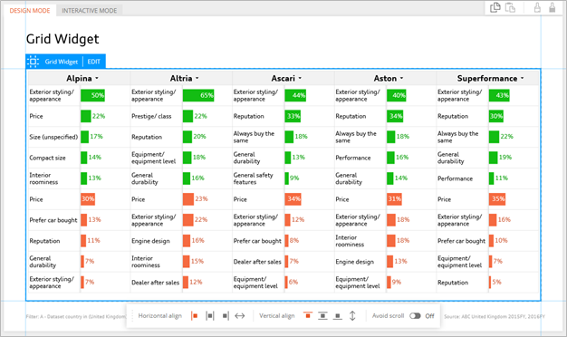
Grid: Using Data from Different Queries

 

This example includes data from separate queries, one for purchase reasons and one for rejection reasons.

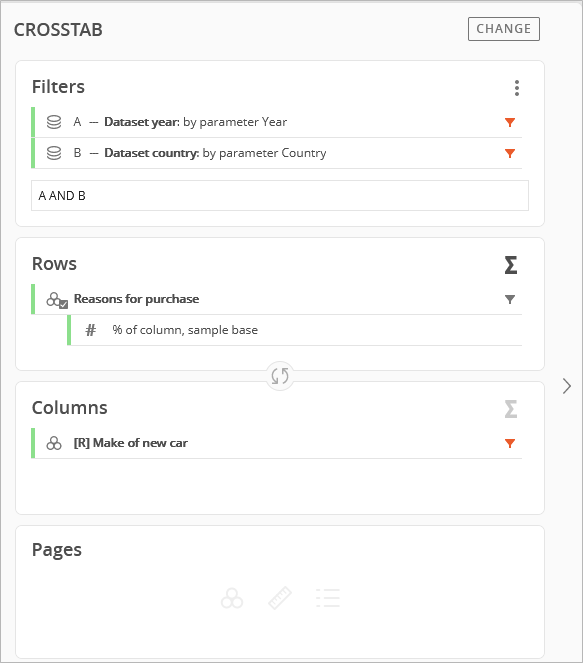
The purchase reasons query uses the make/model purchased question.

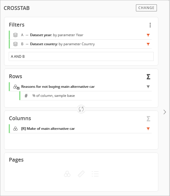
The rejected reasons query uses the make/model considered question.

Assuming there are common, matching make/model labels between the two queries, the labels in the rejection reasons query are matched to the labels in the purchase reasons query.

This is another benefit of using grids. A single table using grids can include data from multiple queries.

 

 

 

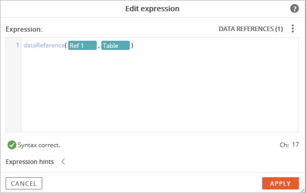
For reference, this is the crosstab setup for the purchase reasons.

 

 

This is the crosstab setup for the rejection reasons.

 

 

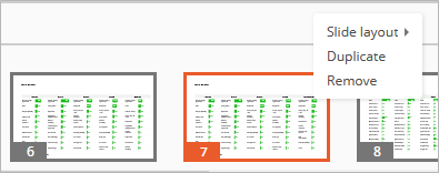
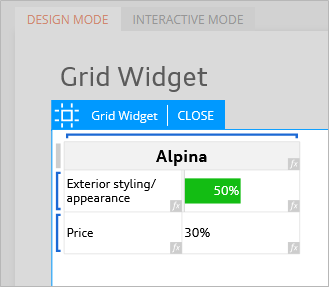
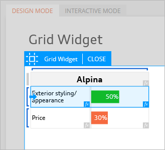
To leverage some of the work that has already done, we will duplicate one of the pages with a previous grid example.

Select the second example that we completed that included the grid with bar charts and purchase reasons.

 

 

After duplicating the page, select the existing grid and click the Edit tab at the top of the grid.

 

Note: It is important to make sure you are working with a duplicate of the existing page, otherwise your previous grid example will be updated and overwritten with the steps included in this example.

 

 

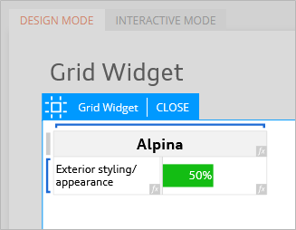
The next step is to edit the Dynamic Row option.

Hover over the left border of the first cell and a blue bracket will appear.

Click the blue bracket to display the menu for the Dynamic Row, then click the EXPR option to open the expression editor.

 

 

The data reference is already linked to the purchase reasons tab, so no changes are needed. As a reminder, this expression is currently setup to sort on the top 10 responses. Edit the expression to sort and display the top 5 responses instead. Change “11” to “6” to display 5 responses. We need to enter 6 instead of 5 because we also are using a filter in the expression to exclude the “Sample total” response in the results. Without the filter, this response would typically appear in the first (top) position in the sorted results since the total sums to 100%.

 

Exit Edit Mode to view the updated grid.

 

 

The updated grid should now show 5 bars sorted in descending order.

Select the grid again and get back into Edit Mode.

 

 

 

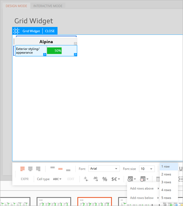
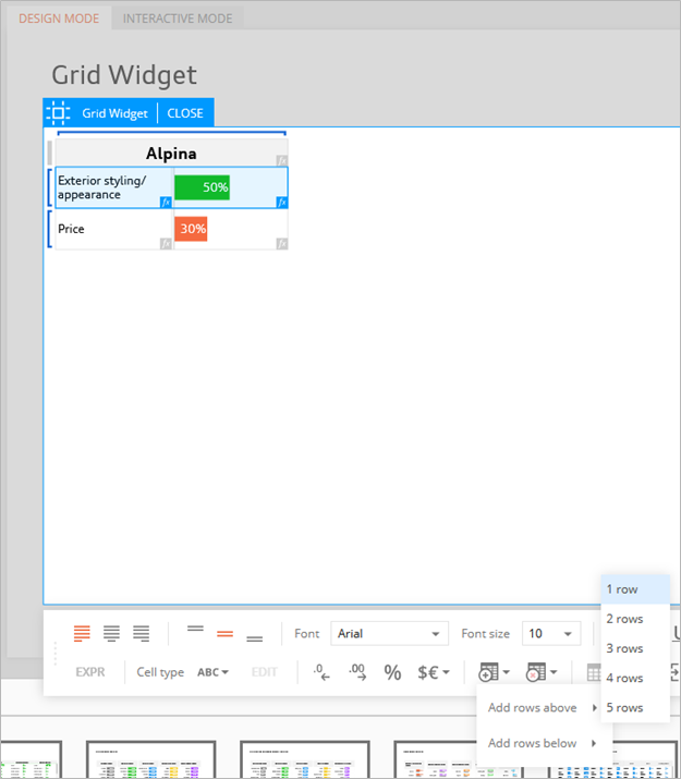
Next, an additional dynamic row needs to be added to the bottom of the grid for the rejection reasons.

 

Select at least one of the cells in the existing row and the toolbar options will appear at the bottom.

Click the icon with the grid and the plus sign.

Select the option to add rows below and add 1 row.

 

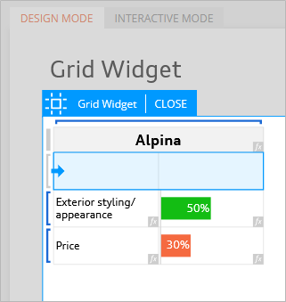
The new row should appear below the original dynamic row.

 

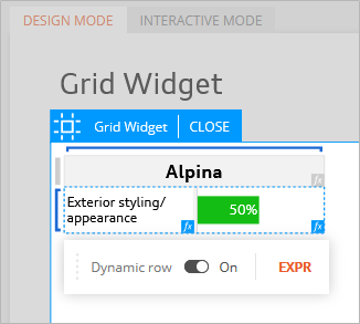
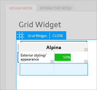
The next step is to turn on the Dynamic Row option for the newly added row.

Hover over the left border of the first cell in the newly added, second row and a blue bracket will appear.

Click the blue bracket to display the menu for the Dynamic Row, then turn it on.

 

Turning on the Dynamic Row option will make the bracket red.

This indicates that the data range for the Dynamic Row will need to be defined.

 

A Dynamic Row is needed because we want to create a reference for the brands listed in the first row and have the rows for the remaining responses populate automatically (and dynamically).

 

After turning on the Dynamic Row, click the Expression option (EXPR) in the menu bar.

 

 

The expression editor window will appear.

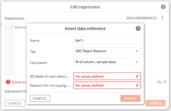
Click the Data References option in the upper-right corner.

 

Follow the prompts to define the data references.

This is where the data range (tab, calculations, and questions) are selected.

 

For this data reference, we want to include alternate vehicle makes and the reasons for not purchasing the makes.

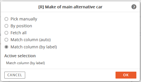
Start by defining how the make of alternate vehicle will be referenced.

 

As a reminder, the setting for dependent rows was turned on previously. This means that the contents in the dynamic rows are connected to the dynamic columns. Notice the match column options are available because the dynamic rows are dependent on the dynamic columns.

 

For this example, we will select the Match Column (Label) option.

This means that the data references for ‘make of main alternative car’ (rejected) will match the ‘make of new car’ (purchased) responses in columns by matching labels of vehicle makes (labels for rejected makes = purchased makes).

 

When working with data references and questions from different question sets, datasets, and/or study families, it is recommended that Match Column (by Label) be used.

Internal codes can vary between study families, so in this scenario codes are not the ideal criteria to create matches on. The Match Column (by Label) ignores the internal coding and uses the actual response label text to create matches.

 

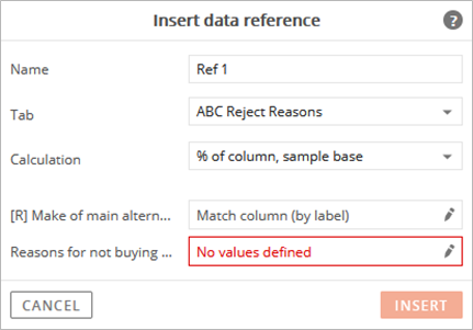
When the remaining expressions are completed, purchase reasons will be shown in the Grid according to the specific make that matches the column selection.

 

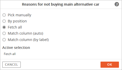
Next, specify the Reasons for not buying (rejection reasons).

 

 

Click the Fetch All option for the Reasons for Not Buying.

 

The Fetch All option is used when we want to include all the responses in the dynamic selection.

 

With this example, Fetch All is being used to include all rejection reasons for each of the matched columns that we previously selected.

 

Confirm the selections, then click the Insert button.

 

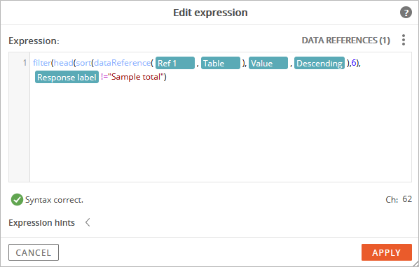
The data reference syntax is shown as correct with a green check mark.

 

 

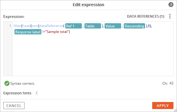
Edit the syntax to add the filter and sorting options.

These are the same options used in the Purchase Reasons expression.

 

Between “filter” and “(dataReferences” type the following:

“(head(sort”

“head” is used with the “sort” command.

head starts at the top of the list.

 

Next, between “Table),” and “Response label”, insert the cursor then hold the SHIFT key + @ to display the available options.

Select Value since we want to add criteria to sort on.

 

After Value is inserted, add a comma, then hold the SHIFT key + @ to display the available options.

 

Select Descending since we want to sort with the highest value first.

Then add a closed parenthesis and a comma “),” after Descending.

 

Next, type in a value for the number of row responses to show after sorting.

Typically, for a Top 5 sort, we would enter 5.

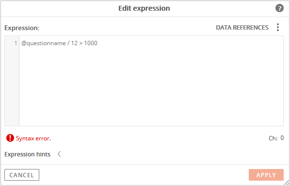
However, because there is an existing filter also being used in the expression, we need to increase the sort value to 6, as “Sample total”, which would be part of the top 5 sort is being filtered.

 

This is the completed, modified expression that includes filtering and a top 5 sort.

Filter(head(sort(dataReference(Ref1,Table),Value,Descending),6),Response label!=”Sample total”)

 

Confirm that the syntax appears correct again with a green check mark.

Click the Apply button.

 

 

 

The bracket on the left border that was previously red is now blue.

The “rejected reasons” data reference for the Dynamic Rows was created successfully.

The next step is to create additional expressions to fill the cells with some content.

 

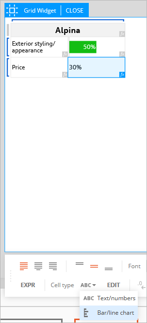
Click on the first (left) cell of the “rejected reasons” row. It will turn blue to indicate that it is currently selected.

A menu bar will appear at the bottom of the page.

Click the EXPR option in the lower-left corner to open the expression editor.

 

An expression is required to display contents in the selected cell.

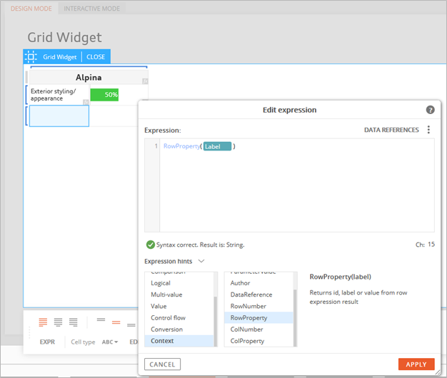
We will create an expression to show the labels for the rejection reasons.

 

 

Expand the Expression Hints, click the Context option, then double-click RowProperty to add it to the expression editor.

 

Hold the SHIFT key + @ to display the available RowProperty options.

Select Label since we want to display the response label of the rejection reasons.

Click Apply to confirm the expression.

 

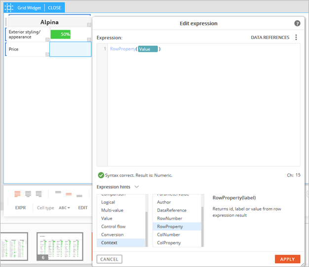
After completing the expression to display the rejection reason labels, select the cell to the right and repeat the previous steps to display the response values for the rejection reasons.

 

Proceed with most of the same steps we used for the left cell to display the row response label.

 

However, after holding the SHIFT key + @ to display the available RowProperty options, select Value instead, since we want to display the actual data value for the rejection reasons.

 

Finish the expression by typing a closed parenthesis “)”.

The syntax will appear as correct with a green check mark.

Click the Apply button.

 

 

The rejection reason value is now shown in the right cell.

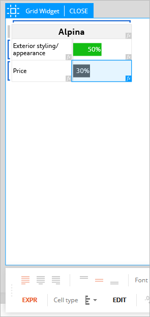
Format it as a percentage by clicking the % icon in the bottom toolbar.

Next, click the .0 icon with the left arrow to reduce the number of decimals shown

 

 

In the bottom menu bar, click the ABC menu to expand the options.

Select the Bar Chart option.

 

This will change the data results (percentage) to a bar chart.

 

 

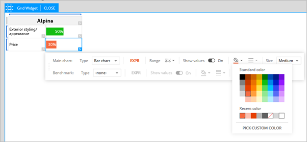
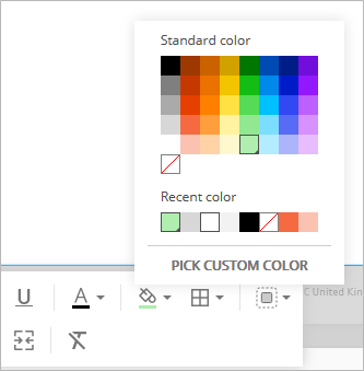
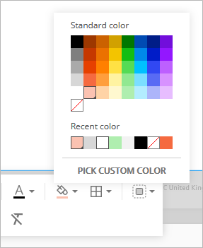
Click the paint bucket icon to specify a different color for the rejected reasons bar chart.

 

After completing the bar format changes, click the Close tab, at the top of the Grid, to exit Edit Mode.

 

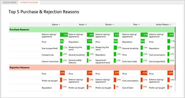
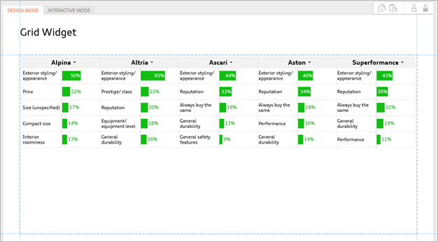
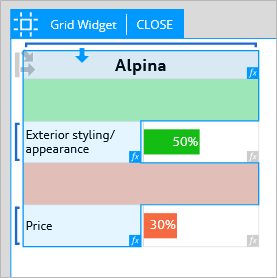
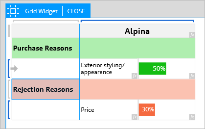
This is the grid with bars that include the top 5 purchase and rejection reasons in descending order.

 

The next steps cover formatting to include extra rows to separate the purchase and rejection bars, so they do not appear as one continuous column of data.

Purchase and Rejection row headers will also be added.

 

Select the Grid and click the Edit tab to get back into Edit Mode.

 

 

Select the first dynamic row that includes the purchase reasons.

 

 

 

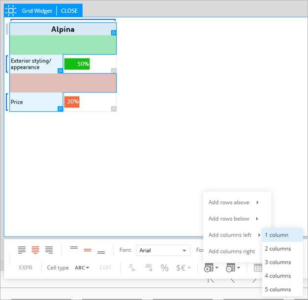
In the bottom menu bar, click the grid icon with a plus (+) sign.

Select Add Rows Above, then choose 1 Row.

 

A new, empty row will appear above the “purchase reasons” row.

 

 

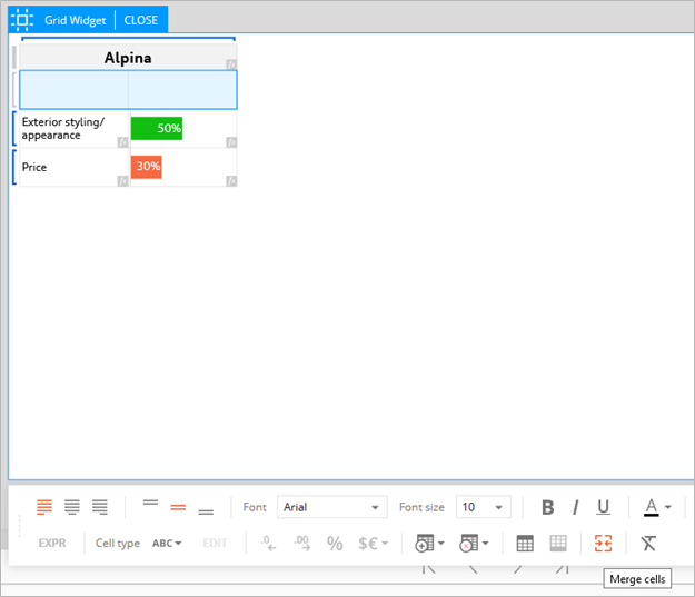
Make sure both cells of the newly added row are selected, then go to the bottom menu and click the Merge Cells icon (two arrows facing each other).

The separate cells will be merged into one.

We will come back to this later to add a label.

 

 

Click the paint bucket icon in the toolbar and select a background color for the newly merged cells.

 

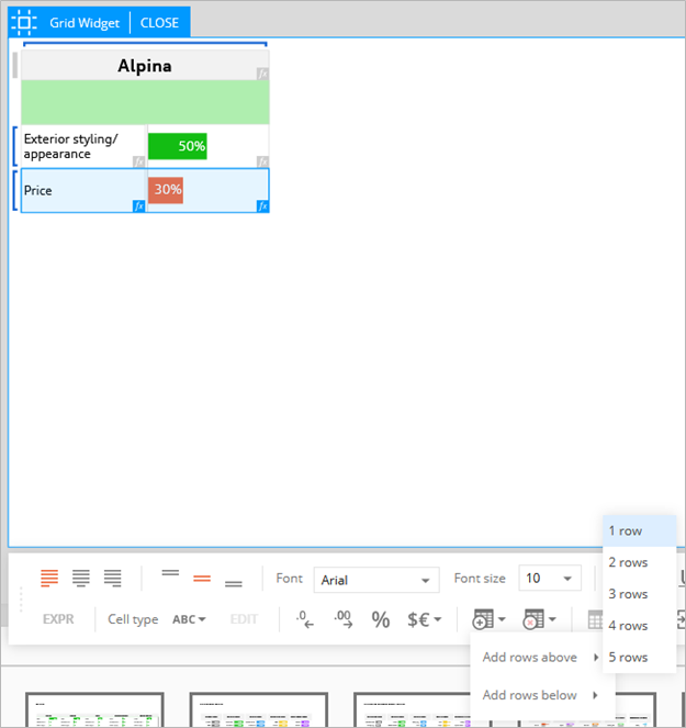
Next, we will add a row between the purchase and rejection reasons rows.

Select the second dynamic row that includes the rejection reasons.

In the bottom menu bar, click the grid icon with a plus (+) sign.

Select Add Rows Above, then choose 1 Row.

 

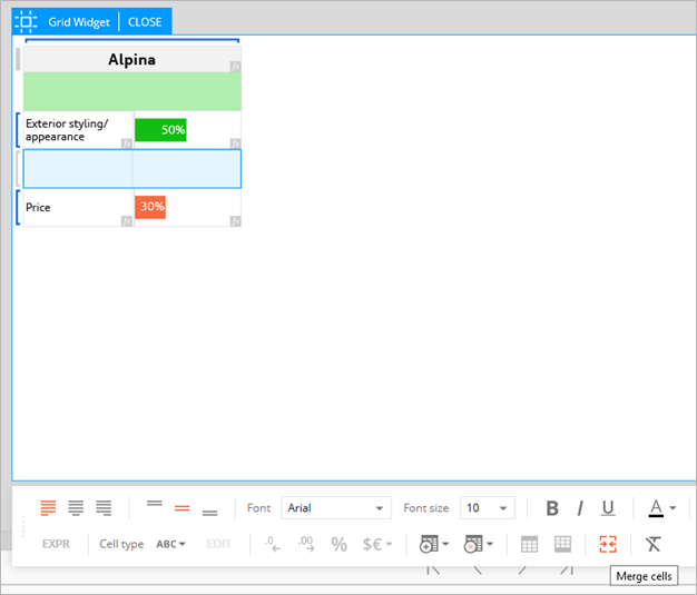
A new, empty row will appear between the purchase and rejection reasons rows.

 

Make sure both cells of the newly added row are selected, then go to the bottom menu and click the Merge Cells icon (two arrows facing each other).

The separate cells will be merged into one.

We will come back to this later to add a label.

 

 

Click the paint bucket icon in the toolbar and select a background color for the newly merged cells.

 

 

Next, we will add a new column to the left.

Select the first column.

 

 

 

In the bottom menu bar, click the grid icon with a plus (+) sign.

Select Add Columns Left, then choose 1 Column.

 

A blank new column will be added to the beginning of the grid.

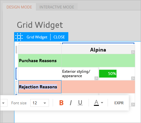
We will add Purchase and Rejection headers here.

 

In the newly added first column, type “Purchase Reasons” in the first row.

Then, type “Rejection Reasons” in the third row.

 

Use the toolbar options to change the formatting of the headers.

 

 

 

The last steps are to resize the column and row widths to fit the grid to the page.

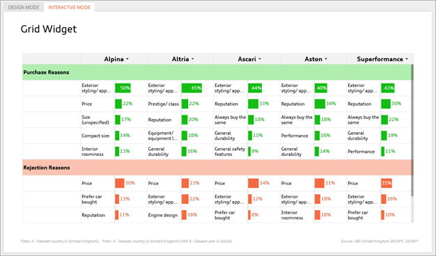
This grid will most likely scroll in the Interactive Mode since there is more content to fit vertically on the page.

 

 

This is the completed example of our purchase and rejection reasons grid.